If you’re up to date with the AI world, you know that Google recently released a model called Inception v3 with Tensorflow.
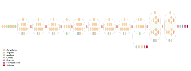
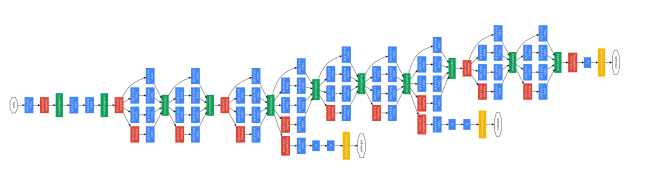
You can use this model by retraining the last layer per your classification requirements. If you’re interested in doing this, check out this speedy 5 min tutorial by Siraj Raval. The namesake of Inception v3 is the Inception modules it uses, which are basically mini models inside the bigger model. The same Inception architecture was used in the GoogLeNet model which was a state of the art image recognition net in 2014.
In this post we’ll actually go into how to program Inception modules using Tensorflow following the details described by the original paper, “Going Deep with Convolutions.” If you’re not already comfortable with convolutional networks, check out Chapter 9 of the Deep Learning book, because we’ll assume that you already have a good understanding of convolutional operations and that you’ve coded some simpler convnets in Tensorflow.
What are Inception modules?
As is often the case with technical creations, if we can understand the problem that led to the creation, we will more easily understand the inner workings of that creation.

Udacity’s Deep Learning Course did a good job introducing the problem and the main advantages of using Inception architecture, so I’ll try to restate them here. The inspiration comes from the idea that you need to make a decision as to what type of convolution you want to make at each layer: Do you want a 3×3? Or a 5×5? And this can go on for a while.
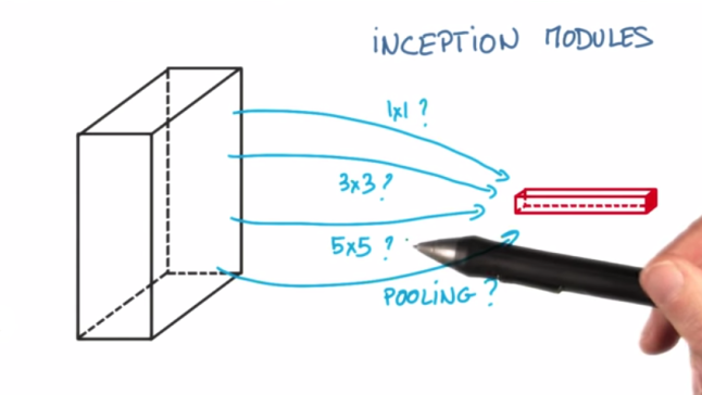
So why not use all of them and let the model decide? You do this by doing each convolution in parallel and concatenating the resulting feature maps before going to the next layer.
Now let’s say the next layer is also an Inception module. Then each of the convolution’s feature maps will be passes through the mixture of convolutions of the current layer. The idea is that you don’t need to know ahead of time if it was better to do, for example, a 3×3 then a 5×5. Instead, just do all the convolutions and let the model pick what’s best. Additionally, this architecture allows the model to recover both local feature via smaller convolutions and high abstracted features with larger convolutions.
Architecture
Now that we get the basic idea, let’s look into the specific architecture that we’ll implement. Figure 3 shows the architecture of a single inception module.
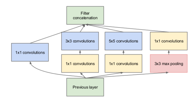
Notice that we get the variety of convolutions that we want; specifically, we will be using 1×1, 3×3, and 5×5 convolutions along with a 3×3 max pooling. If you’re wondering what the max pooling is doing there with all the other convolutions, we’ve got an answer: pooling is added to the Inception module for no other reason than, historically, good networks having pooling. The larger convolutions are more computationally expensive, so the paper suggests first doing a 1×1 convolution reducing the dimensionality of its feature map, passing the resulting feature map through a relu, and then doing the larger convolution (in this case, 5×5 or 3×3). The 1×1 convolution is key because it will be used to reduce the dimensionality of its feature map. This is explained in detail in the next section.
Dimensionality reduction
This was the coolest part of the paper. The authors say that you can use 1×1 convolutions to reduce the dimensionality of your input to large convolutions, thus keeping your computations reasonable. To understand what they are talking about, let’s first see why we are in some computational trouble without the reductions.
Let’s say we use, we the authors call, the naive implementation of an Inception module.
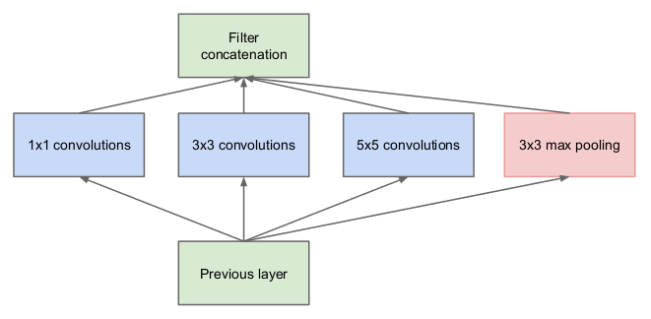
Figure 4 shows an Inception module that’s similar to the one in Figure 3, but it doesn’t have the additional 1×1 convolutional layers before the large convolutions (3×3 and 5×5 convolutions are considered large).
Let’s examine the number of computations required of the first Inception module of GoogLeNet. The architecture for this model is tabulated in Figure 5.
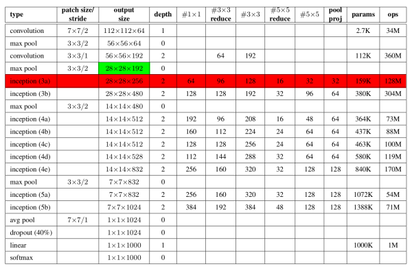
We can tell that the net uses same padding for the convolutions inside the module, because the input and output are both 28×28. Let’s just examine what the 5×5 convolution would be computationally if we didn’t do the dimensionality reduction. Figure 6. pictorially shows these operations.
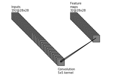
There would be

Wow. That’s a lot of computing! You can see why people might want to do something to bring this number down.
To do this, we will ditch the naive model shown in Figure 4 and use the model from Figure 3. For our 5×5 convolution, we put the previous layer through a 1×1 convolution that outputs a 16 28×28 feature maps (we know there are 16 from the #5×5 reduce column in Figure 5), then we do the 5×5 convolutions on those feature maps which outputs 32 28×28 feature maps.
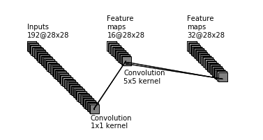
In this case, there would be
![[(1^2)(28^2)(192)(16)]+[(5^2)(28^2)(16)(32)]=2,408,448+10,035,200= 12,443,648\text{ operations.}](https://s0.wp.com/latex.php?latex=%5B%281%5E2%29%2828%5E2%29%28192%29%2816%29%5D%2B%5B%285%5E2%29%2828%5E2%29%2816%29%2832%29%5D%3D2%2C408%2C448%2B10%2C035%2C200%3D+12%2C443%2C648%5Ctext%7B+operations.%7D&bg=ffffff&fg=000000&s=0&c=20201002)
Although this is a still a pretty big number, we shrunk the number of computation from the naive model by a factor of ten.
We won’t run through the calculations for the 3×3 covolutions, but they follow the same process as the 5×5 convolutions. Hopefully, this sections cleared up why the 1×1 convolutions are necessary before large convolutions!
That wraps up the specifics of the Inception modules and hopefully clears up any ambiguity. Now time to code our model.
Tensorflow implementation
Coding this up in Tensorflow is more straightforward than elegant. For data, we’ll use the classic MNIST dataset. We didn’t use the typical crazily formatted version, but found this neat site that has the csv version. The architecture of our model will include two Inception modules and one fully connected hidden layer before our output layer. You’ll definitely want to use your GPU to run the code, or else it’ll will take hours to days to train. If you don’t have a GPU, you can check to see if your model works by using just a couple hundred training steps. Depending on your computer, you might get a resource exhaust error and will have to shrink some of the parameters to get the code to run; in fact, I wasn’t able to use the parameters described in the paper which is why mine are smaller. On the other hand, if your machine can handle more parameters, you’ll be able to make your network wider and/or deeper.
Imported libraries
We’ll use pandas and numpy to preprocess the data and Tensorflow for the neural net.
import pandas as pd
import numpy as np
import tensorflow as tf
Data and preprocessing
Use pandas to import the csv.
train_set = pd.read_csv('mnist_train.csv',header=None)
test_set = pd.read_csv('mnist_test.csv',header=None)
The images, represented by rows in the table, need to be separated from the labels. Additionally, The labels need to be one-hot encoded.
 #get labels in own array
train_lb=np.array(train_set[0])
test_lb=np.array(test_set[0])

#one hot encode the labels
train_lb=(np.arange(10) == train_lb[:,None]).astype(np.float32)
test_lb=(np.arange(10) == test_lb[:,None]).astype(np.float32)

#drop the labels column from training dataframe
trainX=train_set.drop(0,axis=1)
testX=test_set.drop(0,axis=1)

#put in correct float32 array format
trainX=np.array(trainX).astype(np.float32)
testX=np.array(testX).astype(np.float32)
Next, reformat the data so its a 4D tensor.
#reformat the data so it's not flat
trainX=trainX.reshape(len(trainX),28,28,1)
testX = testX.reshape(len(testX),28,28,1)
It’ll be good to have a validation set so we can monitor how training is going.
#get a validation set and remove it from the train set
trainX,valX,train_lb,val_lb=trainX[0:(len(trainX)-500),:,:,:],trainX[(len(trainX)-500):len(trainX),:,:,:],\
                            train_lb[0:(len(trainX)-500),:],train_lb[(len(trainX)-500):len(trainX),:]
I ran into memory issues when trying to test all my data at once, so I created this class that’ll batch data.
#need to batch the test data because running low on memory
class test_batchs:
    def __init__(self,data):
        self.data = data
        self.batch_index = 0
    def nextBatch(self,batch_size):
        if (batch_size+self.batch_index) > self.data.shape[0]:
            print "batch sized is messed up"
        batch = self.data[self.batch_index:(self.batch_index+batch_size),:,:,:]
        self.batch_index= self.batch_index+batch_size
        return batch

#set the test batchsize
test_batch_size = 100
Before we start building models, create a function that’ll compute the accuracy from predictions and corresponding labels.
#returns accuracy of model
def accuracy(target,predictions):
    return(100.0*np.sum(np.argmax(target,1) == np.argmax(predictions,1))/target.shape[0])
Model
It’s good to save our model after training so we can continue training without starting from scratch. This specific command will only work if you’re running linux.
#use os to get our current working directory so we can save variable there
file_path = os.getcwd()+'/model.ckpt'
Set hyperparameters.
- batch_size: training batch size
- map1: number of feature maps output by each tower inside the first Inception module
- map2: number of feature maps output by each tower inside the second Inception module
- num_fc1: number of hidden nodes
- num_fc2: number of output nodes
- reduce1x1: number of feature maps output by each 1×1 convolution that precedes a large convolution
- dropout: dropout rate for nodes in the hidden layer during training
batch_size = 50
map1 = 32
map2 = 64
num_fc1 = 700 #1028
num_fc2 = 10
reduce1x1 = 16
dropout=0.5
Time for the bulk of the work, which will require Tensorflow. Once the graph is defined, create placeholders that hold the training data, training labels, validation data, and test data. Then create some helper functions which assist in defining tensors, 2D convolutions, and max pooling. Next, use the helper functions and hyperparameters to create variables in both Inception modules. Then, create another function that takes data as input and passes it through the Inception modules and fully connected layers and outputs the logits. Finally, define the loss to be cross-entropy, use Adam to optimize, and create ops for converting data to predictions, initializing variables, and saving all variables in the model.
graph = tf.Graph()
with graph.as_default():
    #train data and labels
    X = tf.placeholder(tf.float32,shape=(batch_size,28,28,1))
    y_ = tf.placeholder(tf.float32,shape=(batch_size,10))

    #validation data
    tf_valX = tf.placeholder(tf.float32,shape=(len(valX),28,28,1))

    #test data
    tf_testX=tf.placeholder(tf.float32,shape=(test_batch_size,28,28,1))

    def createWeight(size,Name):
        return tf.Variable(tf.truncated_normal(size, stddev=0.1),
                          name=Name)

    def createBias(size,Name):
        return tf.Variable(tf.constant(0.1,shape=size),
                          name=Name)

    def conv2d_s1(x,W):
        return tf.nn.conv2d(x,W,strides=[1,1,1,1],padding='SAME')

    def max_pool_3x3_s1(x):
        return tf.nn.max_pool(x,ksize=[1,3,3,1],
                             strides=[1,1,1,1],padding='SAME')

    #Inception Module1
    #
    #follows input
    W_conv1_1x1_1 = createWeight([1,1,1,map1],'W_conv1_1x1_1')
    b_conv1_1x1_1 = createWeight([map1],'b_conv1_1x1_1')

    #follows input
    W_conv1_1x1_2 = createWeight([1,1,1,reduce1x1],'W_conv1_1x1_2')
    b_conv1_1x1_2 = createWeight([reduce1x1],'b_conv1_1x1_2')

    #follows input
    W_conv1_1x1_3 = createWeight([1,1,1,reduce1x1],'W_conv1_1x1_3')
    b_conv1_1x1_3 = createWeight([reduce1x1],'b_conv1_1x1_3')

    #follows 1x1_2
    W_conv1_3x3 = createWeight([3,3,reduce1x1,map1],'W_conv1_3x3')
    b_conv1_3x3 = createWeight([map1],'b_conv1_3x3')

    #follows 1x1_3
    W_conv1_5x5 = createWeight([5,5,reduce1x1,map1],'W_conv1_5x5')
    b_conv1_5x5 = createBias([map1],'b_conv1_5x5')

    #follows max pooling
    W_conv1_1x1_4= createWeight([1,1,1,map1],'W_conv1_1x1_4')
    b_conv1_1x1_4= createWeight([map1],'b_conv1_1x1_4')

    #Inception Module2
    #
    #follows inception1
    W_conv2_1x1_1 = createWeight([1,1,4*map1,map2],'W_conv2_1x1_1')
    b_conv2_1x1_1 = createWeight([map2],'b_conv2_1x1_1')

    #follows inception1
    W_conv2_1x1_2 = createWeight([1,1,4*map1,reduce1x1],'W_conv2_1x1_2')
    b_conv2_1x1_2 = createWeight([reduce1x1],'b_conv2_1x1_2')

    #follows inception1
    W_conv2_1x1_3 = createWeight([1,1,4*map1,reduce1x1],'W_conv2_1x1_3')
    b_conv2_1x1_3 = createWeight([reduce1x1],'b_conv2_1x1_3')

    #follows 1x1_2
    W_conv2_3x3 = createWeight([3,3,reduce1x1,map2],'W_conv2_3x3')
    b_conv2_3x3 = createWeight([map2],'b_conv2_3x3')

    #follows 1x1_3
    W_conv2_5x5 = createWeight([5,5,reduce1x1,map2],'W_conv2_5x5')
    b_conv2_5x5 = createBias([map2],'b_conv2_5x5')

    #follows max pooling
    W_conv2_1x1_4= createWeight([1,1,4*map1,map2],'W_conv2_1x1_4')
    b_conv2_1x1_4= createWeight([map2],'b_conv2_1x1_4')

    #Fully connected layers
    #since padding is same, the feature map with there will be 4 28*28*map2
    W_fc1 = createWeight([28*28*(4*map2),num_fc1],'W_fc1')
    b_fc1 = createBias([num_fc1],'b_fc1')

    W_fc2 = createWeight([num_fc1,num_fc2],'W_fc2')
    b_fc2 = createBias([num_fc2],'b_fc2')

    def model(x,train=True):
        #Inception Module 1
        conv1_1x1_1 = conv2d_s1(x,W_conv1_1x1_1)+b_conv1_1x1_1
        conv1_1x1_2 = tf.nn.relu(conv2d_s1(x,W_conv1_1x1_2)+b_conv1_1x1_2)
        conv1_1x1_3 = tf.nn.relu(conv2d_s1(x,W_conv1_1x1_3)+b_conv1_1x1_3)
        conv1_3x3 = conv2d_s1(conv1_1x1_2,W_conv1_3x3)+b_conv1_3x3
        conv1_5x5 = conv2d_s1(conv1_1x1_3,W_conv1_5x5)+b_conv1_5x5
        maxpool1 = max_pool_3x3_s1(x)
        conv1_1x1_4 = conv2d_s1(maxpool1,W_conv1_1x1_4)+b_conv1_1x1_4

        #concatenate all the feature maps and hit them with a relu
        inception1 = tf.nn.relu(tf.concat(3,[conv1_1x1_1,conv1_3x3,conv1_5x5,conv1_1x1_4]))

        #Inception Module 2
        conv2_1x1_1 = conv2d_s1(inception1,W_conv2_1x1_1)+b_conv2_1x1_1
        conv2_1x1_2 = tf.nn.relu(conv2d_s1(inception1,W_conv2_1x1_2)+b_conv2_1x1_2)
        conv2_1x1_3 = tf.nn.relu(conv2d_s1(inception1,W_conv2_1x1_3)+b_conv2_1x1_3)
        conv2_3x3 = conv2d_s1(conv2_1x1_2,W_conv2_3x3)+b_conv2_3x3
        conv2_5x5 = conv2d_s1(conv2_1x1_3,W_conv2_5x5)+b_conv2_5x5
        maxpool2 = max_pool_3x3_s1(inception1)
        conv2_1x1_4 = conv2d_s1(maxpool2,W_conv2_1x1_4)+b_conv2_1x1_4

        #concatenate all the feature maps and hit them with a relu
        inception2 = tf.nn.relu(tf.concat(3,[conv2_1x1_1,conv2_3x3,conv2_5x5,conv2_1x1_4]))

        #flatten features for fully connected layer
        inception2_flat = tf.reshape(inception2,[-1,28*28*4*map2])

        #Fully connected layers
        if train:
            h_fc1 =tf.nn.dropout(tf.nn.relu(tf.matmul(inception2_flat,W_fc1)+b_fc1),dropout)
        else:
            h_fc1 = tf.nn.relu(tf.matmul(inception2_flat,W_fc1)+b_fc1)

        return tf.matmul(h_fc1,W_fc2)+b_fc2

    loss = tf.reduce_mean(
        tf.nn.softmax_cross_entropy_with_logits(model(X),y_))
    opt = tf.train.AdamOptimizer(1e-4).minimize(loss)

    predictions_val = tf.nn.softmax(model(tf_valX,train=False))
    predictions_test = tf.nn.softmax(model(tf_testX,train=False))

    #initialize variable
    init = tf.initialize_all_variables()

    #use to save variables so we can pick up later
    saver = tf.train.Saver()
To train the model, set the number of training steps, create a session, initialize variables, and run the optimizer op for each batch of training data. You’ll want to see how your model is progressing, so run the op for getting your validation predictions every 100 steps. When training is done, output the test data accuracy and save the model. I also created a flag use_previous that allows you to load a model from the file_path to continue training.
num_steps = 20000
sess = tf.Session(graph=graph)

#initialize variables
sess.run(init)
print("Model initialized.")

#set use_previous=1 to use file_path model
#set use_previous=0 to start model from scratch
use_previous = 1

#use the previous model or don't and initialize variables
if use_previous:
    saver.restore(sess,file_path)
    print("Model restored.")

#training
for s in range(num_steps):
    offset = (s*batch_size) % (len(trainX)-batch_size)
    batch_x,batch_y = trainX[offset:(offset+batch_size),:],train_lb[offset:(offset+batch_size),:]
    feed_dict={X : batch_x, y_ : batch_y}
    _,loss_value = sess.run([opt,loss],feed_dict=feed_dict)
    if s%100 == 0:
        feed_dict = {tf_valX : valX}
        preds=sess.run(predictions_val,feed_dict=feed_dict)

        print "step: "+str(s)
        print "validation accuracy: "+str(accuracy(val_lb,preds))
        print " "

    #get test accuracy and save model
    if s == (num_steps-1):
        #create an array to store the outputs for the test
        result = np.array([]).reshape(0,10)

        #use the batches class
        batch_testX=test_batchs(testX)

        for i in range(len(testX)/test_batch_size):
            feed_dict = {tf_testX : batch_testX.nextBatch(test_batch_size)}
            preds=sess.run(predictions_test, feed_dict=feed_dict)
            result=np.concatenate((result,preds),axis=0)

        print "test accuracy: "+str(accuracy(test_lb,result))

        save_path = saver.save(sess,file_path)
        print("Model saved.")
It should take around one hour to train on a 1060 GPU, and you should have a test accuracy of 98.5%. The accuracy is a little disappointing, because simpler convnets do just as well and take much less time to train, like this example from Tensorflow; but MNIST is infamous for being too easy these days, and these modules earned their reputation from a much more difficult classification task (around 1,000 different labels). I hope this post helped explain the magic behind Inception modules and/or that the code aided in your understanding. The full notebook with all the code can be found on my GitHub.

Thanks for your implementation! Always wonder how the 1×1 convolution was suppose to implemented! Cheers.
LikeLiked by 1 person
No problem! I’m happy to hear someone found the post helpful.
LikeLike
Amazing article !! Thanks so much man !
LikeLiked by 1 person
Hi, in the paper, the author mentioned about approximating an ‘optimal local sparse structure’ of a convolutional vision network using readily available ‘dense components’.
In the above, what do ‘optimal local sparse structure’ and ‘dense components’ refers to, and how to they relate?
LikeLiked by 1 person
Hi Leonard. This was the topic I was most confused about when reading the paper, but luckily the authors did a lot of explaining in section 3. The paper they referenced when talking about the motivation behind Inception Modules was about generative neural nets. Those authors found that their edges in their neural net ended up being very sparse, thus they believe that you can create a deep neural net that is very sparse and still be able to represent visual concepts. This would mean that most of the weights inside a deep classification neural net would be close to zero. So how do you do this? Well the authors came up with the inception module, which is very dense (you have 5×5, 3×3, and 1×1 convolutions happening at every layer of the network), but is able to recover the sparse structure of images after training by making most of the parameters near zero.
If that explanation didn’t help, this is what I thought of the first time a read the paper: There are relatively few key features in most images that play a discriminatory role in deciding the class of the photo (most images have a lot of pixels that are not important; just think if you’d be able to recognize a dog if the picture had a green background or a blue background…). For example, we can identify with a high level of confidence the location of a face in an image just by initially looking for edges of the face and then within the boundaries of those edges looking for shadows (also edges) caused by a nose or an eye; this is what the Haar classifier does. Just image how an inception module could do just this. It could first find the the location of the edges with a 5×5 or 3×3 convolution, then it could check for a nose and two eyes in the next layer with the 3×3 and/or 1×1 convolutions, and finally it could give an output.
LikeLiked by 1 person
I found the ‘optimal local sparse structure’ topic confusing too. Is it possible to extract a optimal local sparse structure nearer the top level of the architecture stack before the consolidation into a dense vector?
LikeLike
Hi Henry. Would you elaborate on your question? Each Inception Module has a concatenation before being passed to the next layer, and the extraction I think is happening in the modules and between the modules.
LikeLike
I’ll re-phrase the question. In VGG16/19, before the fully-connected layers, the ‘block5_pool’ is sparse. Is there an equivalent layer in InceptionV3 and if not, is there a way to create one with fine-tuning by adding a sparse generating layer and retraining just the last few layers?
LikeLike
That’s a good question! From looking at the architecture, it doesn’t look like there’s anything special at the end of Inception V3 that would make it sparse. I haven’t checked out VGG16/19, but is there anything before ‘block5_pool’ that’s forcing the structure to be sparse?
LikeLike
Here are the last few VGG19 layers:
block4_pool Tensor(“MaxPool_3:0”, shape=(?, 14, 14, 512), dtype=float32)
block5_conv1 Tensor(“Relu_10:0”, shape=(?, 14, 14, 512), dtype=float32)
block5_conv2 Tensor(“Relu_11:0”, shape=(?, 14, 14, 512), dtype=float32)
block5_conv3 Tensor(“Relu_12:0”, shape=(?, 14, 14, 512), dtype=float32)
block5_pool Tensor(“MaxPool_4:0”, shape=(?, 7, 7, 512), dtype=float32)
flatten Tensor(“Reshape_13:0”, shape=(?, ?), dtype=float32)
fc1 Tensor(“Relu_13:0”, shape=(?, 4096), dtype=float32)
fc2 Tensor(“Relu_14:0”, shape=(?, 4096), dtype=float32)
predictions Tensor(“Softmax:0”, shape=(?, 1000), dtype=float32)
I guess the ReLu activations are generating the sparsity.
LikeLike
Then I suppose you can also add ReLus to get a sparse output. Have you tried?
LikeLike
No. How would you go about it wrt Inception?
LikeLike
If you look at Figure 0 you’ll see the architecture for Inception V3. You can try to mimic what you pasted above in your own implementation of V3. I’m not sure how you’d use the pretrained version of V3, but if you study the slim library in TensorFlow you should be able to figure it out. Best of luck!
LikeLike
Dinesh Vadhia, have u tried the ReLus to get a sparse output?
LikeLike
I have just started exploring tensorflow on my blog. Sushantparabblog.wordpress.com
This post really helped me to understand inception model.
Thanks alot!
LikeLike
Thanks very helpful to understand the GoogLeNet, and also the questions are very interesting¡¡
LikeLike
That was great explanation. Thank you.
I am a bit confused when you compute the number of operations for Inception(3a) . Why do you use 192 ?
5*5*28*28*192*32 = 120,422,400
I would instead do: 5*5*28*28*32 = 627,200
since 192 feature maps will be summed up to 1*28*28 before convolved by 32*5*5 kernels.
Thank you,
Bis.
LikeLike
Awesome Job Sir, Really Appreciate.
LikeLike
if we apply 1×1 convolution on 192@28*28, how does that outputs a 16 28×28 feature maps and on 16*28*28, if we do the 5×5 convolutions on those feature maps how does that outputs 32 28×28 feature maps. Can you please explain this ?
LikeLike
Wish I had found this earlier. Such awesomeness. Thanks man.
LikeLike
Hi, thank you for your tutorial. it is well explained. When I run you notebook, i get the following error. Can you please help me? I have already search on the net but I can’t find a solution. Thanks
ValueErrorTraceback (most recent call last)
in ()
138
139 loss = tf.reduce_mean(
–> 140 tf.nn.softmax_cross_entropy_with_logits(model(X),y_))
141 opt = tf.train.AdamOptimizer(1e-4).minimize(loss)
142
in model(x, train)
110
111 #concatenate all the feature maps and hit them with a relu
–> 112 inception1 = tf.nn.relu(tf.concat(3,[conv1_1x1_1,conv1_3x3,conv1_5x5,conv1_1x1_4]))
113
114
/usr/local/lib/python2.7/dist-packages/tensorflow/python/ops/array_ops.pyc in concat(values, axis, name)
1120 axis, name=”concat_dim”,
1121 dtype=dtypes.int32).get_shape().assert_is_compatible_with(
-> 1122 tensor_shape.scalar())
1123 return identity(values[0], name=scope)
1124 return gen_array_ops.concat_v2(values=values, axis=axis, name=name)
/usr/local/lib/python2.7/dist-packages/tensorflow/python/framework/tensor_shape.pyc in assert_is_compatible_with(self, other)
846 “””
847 if not self.is_compatible_with(other):
–> 848 raise ValueError(“Shapes %s and %s are incompatible” % (self, other))
849
850 def most_specific_compatible_shape(self, other):
ValueError: Shapes (4, 50, 28, 28, 32) and () are incompatible
LikeLike