Reconstructing Artistic Style

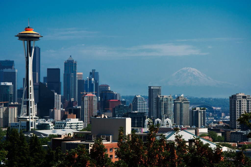
Imagine that you have two images, and you want to create a new image based on some combination of the features of these images. What if you could use the style of one image and the content of the other to create this new image? For example, let’s say you have an image of the Hokusai’s The Great Wave of Kanagawa and a photo of the Seattle skyline, and you want to create a new picture that has the Seattle skyline painted in the pastel, oceanic, and foamy style of The Great Wave of Kanagawa.

This task only seems possible via incredible artistic talent and obscure “vision.” But you can actually develop a systematic method to accomplish this.

In fact, this process can be applied to any pair of style-content images to generate stellar results. The authors of A Neural Algorithm of Artistic Style figured out this process. This post will discuss how they did it.

Basic ideas

Computer vision

If you’ve never dealt with computer vision, it’s worth explaining how an image is represented in a computer. Let’s say your computer displays a black-and-white image. Your computer sees this image as nothing but a 2D map (this is not actually true, because those file extensions like jpeg and png are telling your computer the compression format, but just know that you can get this 2D map from your compressed image). You can think of this 2D map as a grid, where each element in the grid represents a pixel.

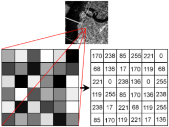
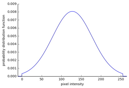
A pixel has an intensity that falls between 0 and 255, where 0 is not intense and 255 is super intense. In our black and white image, an intensity of 0 would be a black, 255 would be white, and anywhere in between would be grey.

A color image in your computer is nothing but three 2D maps, one for each primary color (red, green, and blue).

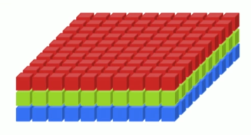
Each map represents the pixel intensities for one of those primary colors. For example, if you had an image that was pure red, you would expect only one of the maps to have non-zero pixels.

Mathematically, we can represent images similarly to how a computer would represent the images using tensors. For a gray-scale image, an image $x$ can be represented by a 2D tensor where $x_{ij}$ is the pixel intensity of position $( i , j )$ of the grid. For a color image, an image $x$ can be represented by a 3D tensor where $x_{ijk}$ is the pixel intensity of position $( i , j )$ of the grid for color $k$ .

Convolutional neural networks

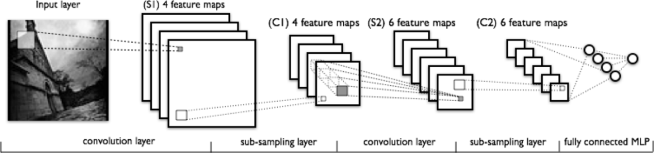
The most important tool for generating novel and stylish images is the convolutional neural network (CNN). To fully understand CNNs will take much more time than what this post allows, but luckily you don’t need to fully understand them to know how they’re used to generate art. A bit of history on how they came to be and a brief summary on how they operate should suffice.

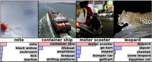
CNNs are traditionally used in image object recognition tasks where images are fed into the CNN, and the CNN outputs a bunch of probabilities about what the main object is in the image (e.g. if you gave a CNN an image of a leopard, you would expect it output a how probability of a leopard).

In the case of image recognition, you can just think of CNN as a mathematical function that takes images as inputs and has probabilities as outputs. But in our case, we actually need to understand a bit more to be able to use them to generate new images.

CNNs achieve their object recognition expertise via transforming the input image through a series of layers, where each layer has a set of feature maps which represents certain features present in the image.

featuremaps1

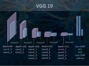
The authors learned that when you pass an image through a deep CNN (they used a modified version of VGG 19, which is a specific type of CNN) trained to perform well for image recognition (their network was trained on ImageNet), you could actually extract the image’s style and content from these feature maps.

A feature map can be represented in two ways: a 2D grid of values or a 1D vector of values. Intuitively, it make sense to think of a feature map as a 2D grid of values, because the feature map really is a 2D map of feature locations that correspond to the locations on the original image.

row-major-2D

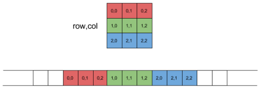
But if we are being pragmatic, we should be able to stretch out this 2D map into a long vector (1D tensor). This is actually how a lot of operations happen when convolutional networks are implemented.

We will be interested in referencing specific feature map values, so we define $F^l_{ij}$ to be the value associated with location $j$ on feature map $i$ in layer $l$ .

Calculus with images

Before moving on to the details of the original paper, it’s important to recognize one more important tool that drives most of the results: using calculus to change images. Ultimately, if there is some function that describes the similarity or distance between two variables (and this function is differentiable), calculus can be used to describe how to change those variables so they are closer to each other. In our case, calculus can be used to change the values of pixels from an image until the image meets some criterion.

For example, let’s say we have two images: Vincent van Gogh’s The Starry Night and a white noise image–this is just an image that has pixel values sampled from a normal distribution that’s centered at 255/2 and truncated at 0 and 255.

trun_norm

The white noise image can be changed to look like The Starry Night by comparing each pixel of the two images, quantifying how much they differ, and then changing the white noise image accordingly.

The difference between two images $y$ and $z$ can be quantified by squaring the difference of pixel intensities between the two images for all pixels

$L(a,b) = \sum\limits_{i,j,k} (y_{ijk} - z_{ijk})^2 .$

This sum of errors is a loss quantifying the difference between two images. This loss is differentiable with respect to the pixels of the white noise image, and thus we can quantify how to change the pixel values in the white noise image to get the two images closer.

Once we change the white noise image to get a little closer to The Starry Night, we can again measure the loss and differentiate to find out what changes to make. This process can be repeated until the white noise image and The Starry Night image are indistinguishable.

Content reconstruction

In order to create new image using a blend of content and style, we first need a procedure/method that creates a new image which has content (i.e. the image scene) that matches the content of some other image; this method is known as content reconstruction. Reconstructing an image from its content can be done using CNNs, and it’s more straightforward than the reconstruction of style.

First, define a set of feature maps that will be used as criteria in content assessment. This is done by choosing a layer $l$ from the model. Next, get the values of these feature maps for a content image $p$ by passing the content image through the model; the feature maps at layer $l$ will be the target feature maps $P^l$ . Next, pass a white noise image $x$ through the model, and get the white noise feature maps $F^l$ . Then, compare the target feature maps with the white noise feature maps using a loss function similar to mean squared error

$L_{content}(p,x,l) =\frac{1}{2} \sum \limits_{i,j}(F^l_{ij}-P^l_{ij})^2.$

Differentiating this loss function with respect to the white noise image will yield derivatives of the loss with respect to pixels of the image. These derivatives can be used to change the white noise image so it has content closer to the content of the content image according to the feature maps in layer $l$ . After the changes to the white noise image have been made, the loss is measured again and changes are made to the white noise image. This is done until the white noise image has a scene that matches the scene of the content image. This procedure can be applied using a set of feature maps from any layer of the CNN.

Reconstructions that use earlier layers in the network preserve pixel details, whereas reconstructions with later layers lose details but preserve salient features (e.g. the reconstruction of an image that contained a house will still contain a house, but it might have something like a blurry window).

Style reconstruction

Reconstructing style of an image is less intuitive than reconstructing content, but it uses the same principles. Like content reconstruction, a set of feature maps $F^l$ is used as criteria in assessment (this time, style assessment) and is predefined. For each feature map inside the set of feature maps, the correlation of that feature map can be found with every feature map in the set. The unnormalized correlation of feature maps $F^l_i$ and $F^l_j$ is the dot product, which yields a scalar $G^l_{ij}=<F^l_i,F^l_j>=F^l_i \cdot F^l_j$ . A matrix $G$ of all feature map correlations for a collection of feature maps is called the Gram matrix

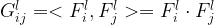
$G(F^l) =\left[\begin{array}{cccc}G^l_{11}&G^l_{12}&\dots&G^l_{1N_l}\\ G^l_{21}&G_{22}&\dots&G^l_{2N_l}\\ \vdots&\vdots&\ddots&\vdots \\ G^l_{N_l1}&G^l_{N_l2}&\dots&G^l_{N_lN_l} \end{array}\right],$

where $N_l$ is the number of feature maps in $F^l$ . It turns out that the original authors were experts at understanding how textures are represented in images. They knew that this Gram matrix would be a good way to define the texture/style of the image.

So, for each layer of a CNN, a Gram matrix can be computed that describes the style of an image. Because the authors were mathematicians, they figured that if we had two images we can get two Gram matrices, compare them with some sort of loss function, and then use calculus with the loss and pixels of one of the images to change that image to have style more like the other. Specifically the loss for a layer $l$ and style image $a$ would be

$L_{style}(a,x,l) =w_l \frac{1}{4N_l^2M_l^2}\sum\limits_{i,j} (G_{ij}^l-A_{ij}^l)^2,$

where $w_l$ is the weight of the loss for layer $l$ (this is a user specified parameter or can be retrieved from a user defined function $W: \lambda \rightarrow \mathbb{R}$ by setting $w_l = W(l)$ ), $G$ is the Gram matrix of the white noise image, $A$ is the Gram matrix of the style image, and $M_l$ is the size of a feature map from layer $l$ .

Style generation can be done using multiple layers of the network to take advantage of different aspects of style picked up by the CNN. To do this, we define a set of layers $\lambda$ that we use to generate the style. Then we define our new style loss to be

$L_{style}(a,x) = \sum\limits_{l\in \lambda}L_{style}(a,x,l).$

The iterative process of changing a white noise image based off derivatives of a loss with respect to the pixels of the white noise image can be used with the style loss to create new images that have a style strikingly similar to the style image.

conv1_1, conv2_1, conv3_1, conv4_1, and conv5_1

The authors figured out that a Gram matrix of an earlier layer in a network describes style at a smaller scale in the image while a Gram matrix of a later layer in the network describes style at a larger scale in the image.

Generating stylish images with content

Images that have the style of one image but the content of another can be generated by jointly changing a white noise image to satisfy style and content criteria simultaneously. To do this, we create a new loss

$L(a,p,x,l_c,\lambda) = \alpha L_{content}(a,x,l_c) + \beta L_{style}(a,x,\lambda),$

where $l_c$ is the layer used to reconstruct content, $\alpha$ is the content weight, and $\beta$ is the style weight. Finally, we use this content-style loss as the criteria to change the white noise image.

The authors had a list of parameters specifying details like the layers used for creating style in the image. Here is that list:

$\lambda = \{\text{conv1\_1, conv2\_1, conv3\_1, conv4\_1, conv5\_1}\}$
$l_c = \text{conv4\_2}$
ratio of content weight to style weight $\frac{\alpha}{\beta} \approx 10^{-3}$
$w_l = \frac{1}{5}, \quad \forall l \in \lambda$ .

The authors also used L-BFGS for optimization, but I found that Adam with a learning rate of about 1-5 can generate aesthetic results in roughly 500 to 2000 iterations.

Conclusions

Seemingly novel images can be generated that incorporate style from one image and content from another. This remarkable achievement uses convolutional neural networks to extract content and style from individual images while using clever loss functions and calculus to iteratively create new images. People have built upon the work of the original authors to create–again–astonishing computer generated images (Deep Dream and CycleGAN to name a few). The future of AI and its influence to our creative processes are very much in flux, and whatever comes next is sure to be extraordinary. Check out my GitHub for implementation of the full method and for code used to generate images in this post.

Reconstructing Artistic Style